|
Concepts
illustrated in the paper
(The
list is expandable. Click on the concept to see its description.)
|
|
Structure:
- Introduction (see example)
- The
Introduction should convey four things. First, what is the question
that the paper asks. Second, why is the question important. Third, how
is the paper going to answer the question. Finally, how is the paper
related to existing work. The introduction is the most important part
of any paper. No one will continue to read any further if the
introduction is confusing or poorly written.
- Data (see
example)
- The
Data section should accomplish three things: First, state the sources
of data. Second, discuss the variables used and how they relate to the
concepts that they are supposed to measure. Finally, present the data’s
descriptive statistics.
- Empirical Results (see example)
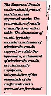
- The
Empirical Results section should present and discuss the empirical
results. The presentation of results is usually done with a table. The
discussion of results typically includes a statement of whether the
results support or refute the hypothesis, a statement of whether
the results are statistically significant, interpretation of the
magnitude of the coefficients and a comment on functional form.
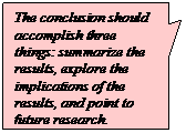
- Conclusion (see example)
- The
conclusion should accomplish three things: summarize the results,
explore the implications of the results, and point to future research.
|
Writing Style:
- Citation Style (see example)
- Use of acronyms (see example)
- The
first time an acronym is used it should be written out, followed by the
acronym in parenthesis.
- Use of first person (see
example)
- It
is acceptable to use first person (I) in an economics paper.
- Coherence (see example)
- Make
each sentence linked to the previous one.
- Tense (see example)
- It
is appropriate to use past tense when describing the construction of
your variables. However, use present tense when referring to tables or
your results.
|
|
Conventions in an Empirical Paper:
- Descriptive Statistics Table (see
example)
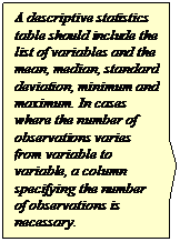
- A
descriptive statistics table should include the list of variables and
the mean, median, standard deviation, minimum and maximum. In cases
where the number of observations varies from variable to variable, a
column specifying the number of observations is necessary. The
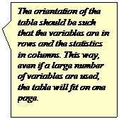
orientation of the table should be such that the variables are in rows
and the statistics in columns. This way, even if a large number of
variables are used, the table will fit on one page.
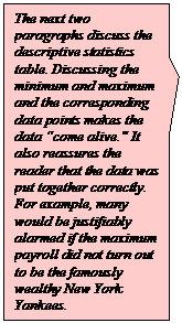
- Discussing Descriptive Statistics (see example)
- Discussing
the minimum and maximum and the corresponding data points makes the
data “come alive.” It also reassures the reader that the data was put
together correctly.
- Rounding numbers in the text (see example)
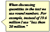
- When
discussing quantities in the text, use round numbers.
- Presentation of regression results (see
example)
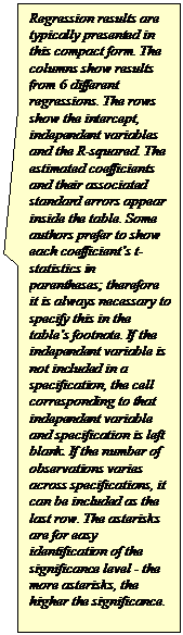
- Regression
results are typically presented in this compact form. The columns show
results from 6 different regressions. The rows show the intercept,
independent variables and the R-squared. The estimated coefficients and
their associated standard errors in parentheses appear inside the
table. Some authors prefer to show each coefficient’s t-statistics in
parentheses; therefore it is always necessary to specify this in the
table’s footnote. If the independent variable is not included in a
specification, the cell corresponding to that independent variable and
specification is left blank. If the number of observations varies
across specifications, it can be included as the last row. The
asterisks are for easy identification of the significance level - the
more asterisks, the higher the significance.
- Converting variables to convenient units (see
example)
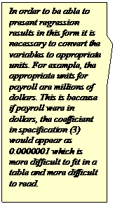
- In
order to be able to present regression results in a compact and
readable form, it is necessary to convert the variables to appropriate
units. For example, the appropriate units for payroll are millions of
dollars. This is because if payroll were in dollars, the coefficient in
specification (3) would appear as 0.0000001 which is more difficult to
fit in a table and more difficult to read.
- Interpreting estimated coefficients (see
example)
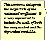
- It
is very important to include the units of both the independent and the
dependent variables.
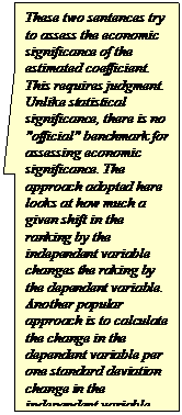
- Assessing economic significance (see example)
- Assessing
economic significance requires judgment. Unlike statistical
significance, there is no "official" benchmark for assessing
economic significance.
|
Other:
- Title (see example)
- The
title should concisely express what the paper is about. It can also be
used to capture the reader's attention.
- Searching for existing literature (see example)
- EconLit
is the most commonly used database for searching published papers in
Economics. Working papers can be found via IDEAS, SSRN,
NBER or even google.
- Effect vs. affect (see example)
- "Effect"
is usually a noun (that is, it could be preceeded by "the").
"Affect" is usually a verb.
- Appeal to authority (see example)
- It
is appropriate to cite other studies when justifying the use of a
variable or technique. This also makes the comparison to other work
easier.
- Acknowledge shortcomings of data (see example)
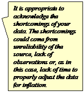
- It
is appropriate to acknowledge the shortcomings of your data. The
shortcomings could come from unreliability of the source, lack of
observations or, as in this case, lack of time to properly adjust the
data for inflation.
|
|
|
Does
pay inequality within a team affect performance?
Tomas Dvorak*
|

|
|

|
1. Introduction
The business of sports draws considerable attention from the media and the
general public. Fans and sports writers frequently speculate about the
effects of money on athletic performance. There is general agreement that
more financial resources usually lead to better athletic performance. In team
sports, higher pay can be used to lure better players from other teams and
therefore improve performance. However, performance can
also be affected by pay inequality among players within a team. On the one
hand, pay inequality could have a negative effect because it may hinder
cooperation among team members. In many sports, team cooperation is critical
for good performance. If pay inequality creates tensions or animosity among
team members, performance is likely to suffer. On the other hand, inequality
could have a positive effect on performance by providing incentives. The
prospect of a very large salary could be a powerful drive behind an athlete’s
performance. Pay inequality might also enhance performance if low paid
players learn from high paid players. This would happen when pay inequality
is associated with skill inequality. For example, if a highly paid superstar
can teach other players, the overall performance of a team may improve. Given
that arguments can be made both ways, it is not surprising that there is
little agreement on the effects of pay inequality on team performance. The
purpose of this paper is to determine whether, on balance, the effect of pay
inequality on performance is positive or negative.
|

|
|
|
Understanding the effect of pay inequality on a team’s performance is important
for at least two reasons. First, team managers can use this information to
make decisions about which players to hire. For example, should they hire one
expensive superstar and two inexpensive players, or three medium-priced
players? If we find that pay inequality leads to poor team performance, then
the team may perform better with three medium-priced players than one
superstar and two low-priced players. Second, because salaries are a large
part of contract negotiations between player associations and team owners,
understanding the effects of pay inequality on performance can help determine
optimal policies. For example, if pay inequality has a negative effect on
performance, an argument for a higher minimum salary could be made.
|

|
|

|
There are a number of studies
that look at the effects of pay inequality on performance. DeBrock, Hendricks
and Koenker (2004) study the effects of pay inequality on performance in
Major League Baseball (MLB) . They find that pay
inequality is associated with poor performance. Frick, Prinze and Winklemann
(2003) look at the effects of pay inequality in all four major leagues in
North America. They find that inequality improves team performance in
basketball and worsens team performance in baseball. They find no
statistically significant effect of inequality on performance in football and
hockey.
|
|
|

|
This paper looks at the effects of
inequality on performance in MLB. It differs from that of DeBrock, Hendricks
and Koenker (2004) in that it uses the most recent data. While the previous authors
use data from 1985 through 1998, I use data from the latest two seasons: 2003
and 2004. Another difference is that I use a different measure of pay
inequality. Rather than the Herfindahl index, I use the percentage of payroll
earned by the best paid 20% of players. I chose the share earned by the top
20% players for two reasons: it is somewhat easier to calculate, and its
magnitude is easier to interpret.
|
 
|
|
|
2. Data
The data on pay inequality was constructed in the following way. From the USA
Today salary database, I collected annual salaries for each player in all MLB
teams during the 2003 and 2004 seasons. I summed the salaries of all players
for each team and each season to obtain the total payroll. The active roster
in baseball is 25, but the database includes salaries of disabled players as
well. Therefore, the number of players for each team ranges from 25 to 31. As
the measure of pay inequality, I calculated the percentage of payroll earned
by the highest paid 20% of players. For example, for a 30 player team I
summed the salaries of the highest paid 6 players and divide that amount by
total payroll. If every player earned the same amount, the best paid 20%
would earn exactly 20% of the payroll. When pay is unequal, this measure is
higher than 20%. The higher the share of payroll earned by the top 20% of
players, the higher the pay inequality.
To measure performance I use the percentage of games won in the regular
season. This data comes from BaseballReference.com. It does not include
performance during league championships or the World Series. However, with
162 games per regular season, the winning percentage can be regarded as a
reasonable measure of performance. This is
also the measure used by DeBrock, Hendricks and Koenker (2004).
|
  

|
|
|
In addition to pay inequality and performance, I use data on the total
payroll of each team. This is a measure of financial resources which could be
an important determinant of performance. I measure payroll in current dollars
and do not adjust for inflation. While
2003 dollars are not exactly comparable to 2004 dollars, 2003 inflation was
low enough not to influence the results significantly.
Table 1 shows the descriptive
statistics of each variable. In the first row we see that on average the highest
paid 20% of players earn about 61% of the total payroll. This implies that on
a 30 player team, the six best paid players earn more than the remaining 24
combined. According to this measure, the team with the most equitable pay is
the New York Yankees during the 2003 season when the top 20% of players
earned only 42% of total payroll. The team with the highest inequality was
the Colorado Rockies during the 2004 season. On that team, five players
earned more than 78% of the team’s total payroll.
The second row in Table 1 shows that the average winning percentage is 50%
which has to be the case since for every game won there is a game lost. The
Detroit Tigers have the lowest winning percentage in the data with only 26%
of games won during the 2003 season. The maximum winning percentage in the
data is for the St. Louis Cardinals, who won nearly 65% of their games during
the 2004 season. Finally, the last row in Table 1 shows that the average
payroll is about 70 million dollars. The range of payroll is quite striking. It goes from less than 20 million dollars for the Tampa Bay
Rays to over 184 million for the New York Yankees.
Table 1: Descriptive Statistics
|
|
mean
|
median
|
st.dev.
|
min
|
max
|
|
Top20share
(in %)
|
61.0
|
61.4
|
8.0
|
42.2
|
78.3
|
|
Games
Won (in %)
|
50.0
|
51.6
|
8.2
|
26.5
|
64.8
|
|
Payroll
(in mil. USD)
|
70.0
|
65.3
|
30.3
|
19.6
|
184.2
|
|
|
|
|
3. Empirical Results
I estimate three different specifications. The dependent variable in each
specification is performance, as measured by the percentage of games won. Pay
inequality and total payroll are the independent variables. Table 2 shows the
results. In the first specification, I regress performance on the share
earned by the top 20% of players. The coefficient on the share of top 20% is
negative and statistically significant. This indicates that teams with higher
pay inequality tend to win fewer games. A one percentage point increase in
the share of payroll earned by the top 20% of players is associated with
about half of a percentage point decline in the percentage of games won.
Table 2: Regression Results
|
Dependent variable: winning percentage (in %)
|
|
|
(1)
|
(2)
|
(3)
|
|
Intercept
|
77.3
(7.43)**
|
59.9
(9.51)**
|
37.35
(15.37)*
|
|
Top20share (in %)
|
-0.45
(0.12)**
|
-0.27
(0.13)*
|
-0.28
(0.13)*
|
|
Payroll (in mil. USD)
|
|
0.10
(0.04)**
|
|
|
Log of Payroll
|
|
|
7.09
(2.43)**
|
|
R-squared
|
0.19
|
0.29
|
0.29
|
|
Adjusted R-squared
|
0.18
|
0.26
|
0.27
|
|
Number of observations is 60.
Standard errors are in parentheses.
** significant at 1%, * significant at 5%
|
In the second specification I include total payroll as an independent
variable. Payroll is a measure of the financial resources which can affect
performance - the higher the payroll, the higher the quality of players and,
generally, the better the performance. Therefore, including payroll may
increase the precision of the estimated coefficient on pay inequality. More
importantly, it is possible that pay inequality is correlated with total
payroll. If low payroll teams tend to have more pay inequality, then the
coefficient on pay inequality in specification (1) is biased. Indeed, the
correlation coefficient between the share earned by the top 20% of players
and total payroll is -0.5. Teams with high pay inequality may perform worse
not because of pay inequality, but because they are also the teams with a
lower payroll. Therefore, in order to measure the effect of pay inequality on
performance, I need to control for total payroll.
Once I control for total payroll, the coefficient on the share of the top 20%
remains statistically significant but the magnitude drops substantially. Holding payroll constant, a one
percentage point increase in the share earned by the highest paid 20% is
associated with a 0.27 percentage point decline in the percentage of games
won. The impact of inequality on
performance does not seem enormous. For example, a five percentage point
increase in inequality for the team with median inequality would shift the
team up 13 spots in the inequality ranking, but its performance ranking would
drop by only 2 spots. The coefficient on total payroll is positive and
statistically significant. A one million dollar increase in total payroll is
associated with about 0.1 percentage point increase in the percentage of
games won. This indicates that greater financial resources tend to improve
performance. Adding payroll as an independent variable led to an increase in
R-squared from about 0.19 to 0.29.
Finally, in specification (3) I include the logarithm of payroll instead of
payroll. I want to verify that the result in specification (2) is robust to
different functional forms. In addition, the effect of an additional one
million dollars may be smaller for a team with a 100 million payroll than for
one with a 20 million payroll. Thus, including payroll in logarithm seems
appropriate. The coefficient on the share of the top 20% remains
statistically significant with roughly the same magnitude. The log of payroll
is statistically significant. A one percent increase in payroll is associated
with about 0.07 percentage points increase in the percentage of games won.
|
|
|
|
4. Conclusion
The analysis in this paper shows that pay inequality within MLB teams has a
negative effect on performance. The effect remains statistically significant
even after controlling for total payroll. The result is the same as that of
DeBrock et al. (2004) who use data from 1985 through 1998. My paper confirms
their finding using the most recent data and using a different measure of pay
inequality.
The fact that pay inequality leads to worse performance implies that managers
should strive for pay equality in their teams. For example, instead of hiring
two low-priced players and one superstar, performance may be better if three
medium-priced players are hired. Given these results, it is surprising that
there is not a more equal distribution of pay in baseball. One possible
explanation is that managers may care about attendance as well as winning.
They may be willing to sign up an expensive superstar who will attract fans
even though it will increase pay inequality and may hinder performance.
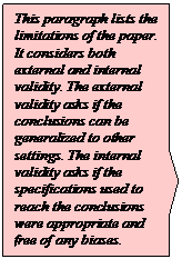
The conclusions above are subject to a number of limitations. First, it is
unclear to what extent the results can be generalized to other sports. Each
sport requires a different degree of cooperation among team members. Therefore,
the relationship between pay inequality and performance is likely to differ
across sports. Second, the error terms for each team could be correlated over
time. For example, if a team wins a lot of games one year given its payroll
and pay inequality, that team is likely to win a lot of games the next year
as well. Therefore, the estimation procedure may need to correct for this
autocorrelation. Finally, there may be other variables that affect
performance, e.g. coach salary or quality of training facilities. Including
these in the regression would increase the precision of my estimates as well
as eliminate potential omitted variable bias.
The channels through which pay inequality affects performance are not clear.
I can think of two possibilities. One is that pay inequality leads to
tensions within the team and impairs performance. The other possibility is
that baseball requires players of similar quality. Pay inequality is probably
associated with skill inequality, and it may be the skill inequality that
drives down performance. An excellent pitcher cannot win the game when the
outfielders cannot catch or throw. It may be possible to distinguish these
two channels empirically. Using statistics on individual player skill level,
one could construct a measure of skill inequality for a team and include it
as an additional control. The coefficient on pay inequality in that case
would capture the effect of pay inequality on
performance while holding skill inequality constant. A negative impact of pay
inequality would then support the idea that pay inequality leads to tensions
which affect performance. This investigation, however, is left for future
research.
|

|
|

|
References:
DeBrock,
Lawrence, Wallace Hendricks, and Roger Koenker. 2004. Pay and performance:
The impact of salary distribution on firm-level outcomes in baseball. Journal
of Sports Economics 5 (August): 243–261.
Frick,
Bernd, Joachim Prinz, and Karina Winkelmann. 2003. Pay inequalities and team
performance: Empirical evidence from the North American major leagues. International
Journal of Manpower 24: 472-491.
|
|
|

|
Appendix:
Data
with documentation and results: MLB.xls
|
|
|
|
(back to the top)
|
|
|
* I would like to thank Mary Mar, Youghwan Song, Stephen
Schmidt and two anonymous referees for their helpful comments. I am also
grateful to many Union College students for their useful feedback.
|