Measuring the Rotation Curve and Mass of the Milky Way

Introduction

(This lab was initially posted at the Haystack SRT web page. Click here to see the original.)

Neutral Hydrogen atoms have an emission line at a frequency of 1420.4 MHz, or a wavelength 21 cm. This emission line has proven to be an extremely useful probe for mapping the interstellar medium of the Milky Way Galaxy (or of any galaxy, for that matter). The interstellar gas of the Milky Way Galaxy is ~90% Hydrogen, by number of atoms, and most of the interstellar gas is relatively cold (~100 K) so the Hydrogen atoms are mostly in the ground state. The 21-cm line is due to a spin flip of the electron in Hydrogen atoms in the ground state orbital. This transition is forbidden and so the photons are not easily absorbed by another Hydrogen atom. Additionally, at a wavelength of 21 cm, these photons are also not absorbed by interstellar dust, which blocks our view at optical wavelengths. Because there are so many Hydrogen atoms in the Galaxy, the strength of the total emission along any line of sight in the plane of the Galaxy is significant. And, because this radiation is not absorbed easily, we can detect the emission from Hydrogen atoms far across the galaxy.

One exceptionally clever application of the 21-cm line observations, which you will do in this lab, yields a determination of the rotation curve of the Milky Way (the rotation speed vs. distance from the center), which, in turn, leads to a measure of the mass of the Milky Way Galaxy. The results, even as performed with our simple 2-meter telescope, are enlightening.

Timing of Observations

In the Fall, the galactic plane is up in the late afternoon.

Get Familiar with SRT_Plotter

Lab Procedure Instructions

Analysis of the Data

Procedure Using the SRT:

In advance of the observation, write a command file to:
1. Move the telescope to Galactic 10 0 (i.e. at Galactic longitude 10^o, or 10^o away from the center of the Galaxy, and latitude 0^o, which is in the Galactic plane) and perform a switching observation with offsets one beamwidth to either side of the Galactic plane (Galactic 10 8 and Galactic 10 -8) for a total of 60 scans.
2. Move the telescope to Galactic 20 0 and perform switching with offsets at Galactic 20 7 and Galactic 20 -7 for 60 scans.
3. Do similar switching observations for positions every 10 degrees in Galactic longitude up to Galactic 80 0.

At the time of the observation:
1. Turn on the computer and ground controller box and click on the SRT icon.
2. Click “record” and input a data file name.
3. Set the frequency to 1420 MHz, mode 4 (this has 3 times the bandwidth as mode 1).
4. Move to a blank area of the aky and do a Tsys measurement.
5. Input pointing offset established from previous labs.
6. Click on “Rcmdfl” and type in the name of your command file. Make sure that you get confirmation in the lower part of the SRT display of this filename. Watch the screen, taking note of the appearances of yellow crosses and the “cmd” positions, to ensure that the program is doing what you expect it to.
7. When done remember to: stop recording data, click on "Stow", and after the telescope has reached 'stow' to close the program. Transfer your data file to your flashdrive, shut off the computer, and turnoff the controller box.

Analysis of Data:

1. Open SRT_Plotter, Click "open file" and "browse" to find your data file.
2. Click "Delete End Channels," choose "select all," and use the mouse and the left button to select an area containing the data in the end channels on the left and on the right. Click on "Delete Selected End Channels".
3. Click "Average Blocks of Data" to average all the scans of Galactic 10 0. Also average all the data of the off-source scans to either side of Galactic 10 0.
4. Repeat step 3 for all the other Galactic longitudes.
5. Click “Subtract Background.” For data block “A” click on the average of the “Galactic 10 0” data and for data block “B” click on the average of off-source data block at this longitude.
6. Repeat step 5 for each Galactic longitude.
7. Select the first “SUB” block. This should then show the final data block for Galactic longitude 10^o.
8. In the pull-down menu that says “Plot Channels” select “Plot Velocities.”
9. Note the flat-baseline and the range of the emission (with antenna temps greater than the baseline). Identify the highest-velocity point of the range of the emission. You can move your cursor to that point and read velocity (the x-coordinate). Record this value in your data table along with the Galactic longitude.
10. Right click in the graph window to save a jpeg file of the plot.
11. Repeat steps 7-10 for the other Galactic longitudes.
12. For each Galactic longitude position (10^o to 80^o):
-Convert this minimum frequency to a recessional velocity using the Doppler shift formula (f_em-f_obs)/f_obs = V_rec/c, where f_em is the frequency that the radiation was emitted at, which is 1420.4 MHz, and f_obs is the frequency that you observed.
This velocity is, now, the V_max along that line of sight,
-Calculate the orbital velocity of this gas (using Eq. 2),
-Calculate the galactocentric distance of this gas (using Eq. 1),
13. Plot the rotational velocity vs. galactocentric distance.
14. Is the velocity vs. radius relation Keplerian (meaning that v² ∝ 1/r)? Keplerian velocity curves result when all the mass is at the center (as in the Solar System). If your data suggests that Galaxy rotation curve is not Keplerian, go to #11.
15. Use Newton's Universal Law of Gravity and your data to calculate the amount of mass inside each of your galactocentric radii. Roughly describe the relation between the enclosed mass and R (especially for the larger radii)? How does this compare with the distribution of star light, which decreases with R as an exponential?

Explanation of Rotation Curve

First, note that the emission line goes to fairly large positive velocities, and not much negative. The reason for this is that you pointed the telescope where there was gas whose orbit about the center of the galaxy gave it a velocity relative to the Sun that was recessional. In the figure below, the line of sight through the galaxy when looking at some non-zero galactic longitude is delineated. (Galactic Longitude is defined as the angle of a line of sight in the plane of the Galaxy relative to the line of sight towards the center of the Galaxy.)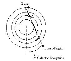

The gas in the plane of the galaxy follows circular orbits. So, at each point along the line of sight the gas has a component of velocity that is along the line of sight and is directed away from the Sun. The Sun also has a component along the line of sight, but all points interior to the Sun have a larger fraction of their orbital velocity along the line of sight than does the Sun. So, all the gas at galactic radii closer than the Sun’s should appear redshifted.
Now note that the gas along the line of sight that is closest to the Galactic center has a motion that is entirely along the line of sight. This gas, then, is responsible for the largest redshifted velocities in the emission. The distance of this gas from the center is easy to determine, using simple geometry. The line of sight at this point is tangent to the circular orbit of this gas, and so the line from the galactic center to this gas is perpendicular to the line of sight.

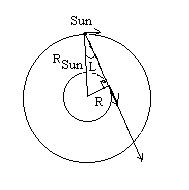
We therefore have a right triangle, with the galactic longitude, L, being the angle opposite the line representing the distance of this gas from the center. If R_Sun is the distance of the Sun from the Galactic Center, then, sinL = R_gas/R_Sun or R_gas = R_SunsinL (Eq. 1)
The distance of the Sun from the Galactice Center is believed to be R_Sun = 8.0 kpc.

So,you need to identify the largest velocity seen in the 21-cm emission at each galactic longitude. The redshift velocity of this gas will be its orbital velocity minus the component of the Sun’s velocity along the line of sight, which is V(Sun)sinL. So, if Vmax is the maximum observed velocity in the 21-cm emission along the line of sight for galactic longitude L, then, V_max = V_gas – V_SunsinL, and so the orbital velocity of the gas is: V_gas = V_max + V_SunsinL. (Eq 2) The Sun's orbital speed is, V_Sun = 220 km/s.