Statistics & Uncertainty

Precision versus Accuracy

In an ideal measurement all trials produce identical values. But in practice this is almost never the case; especially when we try to improve on the precision of the measurement by conducting new experiments. To remedy this reality we perform as many trials as we can in order to convince ourselves that the variation in the values that we obtain are "unavoidable". We then use theory of probabilities and statistics to determine a most trustworthy result based on all of these trials. This process could be just a simple averaging or a more complicated correlation calculation. The accuracy of our measurement depends on how well repeated trials reproduce the same result. Of course, this accuracy depends both on the cleverness of our procedure as well an on the reliability of our measuring apparatus.

The issue of precision is separate from accuracy. Highly precise results often depend a great deal on the high quality of instruments employed in the measurement. For example, if we measure the length of a table with a ruler that is calibrated in inches, then the precision of our measurement cannot be better than 1 inch. The same experiment performed with another ruler that is calibrated in millimeters will give a more precise result. There are times, however, that a clever procedure could produce results with high precision despite the inadequacies of the measurement tools. (An example of this is when we determine wavelength of monochromatic light using a pinhole and a common meter stick in a diffraction measurement.)

The "goodness" of the results not only depends on both its precision and accuracy, but it is also very subjective. It all depends on what we want to do with the results and on what the measurement is all about. As a clever friend once pointed out: "The age of the universe given to a factor of 2 is impressive. The speed of light given to the third decimal place, only, can cause all kinds of problems." Our current estimates suggest that the universe is about 15 billion years old (for a time- line story of the universe, beginning from The Big Bang, see PBS's Mysteries of Deep Space). That is quite a long time for almost any process that we know of. So, even if we are off by a few billion years, this will have no significant effect on anything. On the other hand, we currently use light (electromagnetic waves) regularly in telecommunications. Timing is a very important part of this and its effectiveness greatly depends, among other things, on how precisely (and of course accurately) we know the value of the speed of light. According to National Institute of Standard's web site on Physical Constants this value is known to be: 299 792 458 m/s^-1. Now, consider the signal that your handheld GPS is sending to the satellites, which do the triangulation calculation in order to determine your position. Each satellite is roughly 20 kilometers away. It determines the distance to your location by multiplying the time that it takes the signal (electromagnetic wave, i.e. light) to travel by the speed of light. The difference between a value of 299 792 458 m/s and 299 700 000 (roughly 1 part in 300) translates to a distance measurement difference of 60 meters! For a description of how Global Positioning System works see The Aerospace Corporation's site on GPS and the other sites quoted there.

Error versus Uncertainty Estimation

In analysis of experimental physics we use the word "error" to mean something different from its standard (common) meaning. According to Oxford English Dictionary, the word error was first used to mean wandering and getting off the course. In our every day language error most commonly means mistake. But in physics, as in most fields of applied mathematics it is used to mean deviation from true value.

Below is how Encyclopedia Britannica on-line defines this use of the word error:

In applied mathematics, the difference between a true value and an estimate, or approximation, of that value. In statistics, a common example is the difference between a population mean and the mean of a sample drawn from that population. In numerical analysis, round-off error is exemplified by the difference between the true value of the irrational number π and the value of rational expressions such as 22/7, 355/113, 3.14, or 3.14159. Truncation error results from ignoring all but a finite number of terms of an infinite series. For example, the exponential function e^x may be expressed as the sum of the infinite series

stopping the calculation after any finite value of n gives an approximation to the value of e^x that will be in error, though this error can be made as small as desired by making n large enough.

The relative error is the numerical difference divided by the true value; the percentage error is this ratio expressed as a percent. The term random error is sometimes used to distinguish the effects of inherent imprecision from so-called systematic error, which may originate in faulty assumptions or procedures.

So, when we talk about experimental error we are not referring to blunders or mistakes in the experiment. Instead, we are saying that our final result is only an approximation to some "true" value. Our conjecture that our result is not the "true" value is, of course, based on the fact that different trials have produced varying results. What we call the final value is based on some kind of average of all the trials. In most cases, then, it is fair to consider the departure of these trial values from their average value a measure of our confidence in the "trueness" of our final result. For example, if in some experiment we find that our trials always produce the same exact value, then we feel fairly certain that our result is the true value (within its limit of precision, of course!). On the other extreme, if the trial values wander all over, then we say that our experiment has failed to produce a reliable result.

The method that physicists use for estimating the reliability of their result, or if you will the uncertainty in its trueness, is called error analysis. It is important to note that although almost all error analysis schemes employ mathematical tools of probability theory, they are not exact. This is because one does not know, a priori, why different trials produce different values. As a result, all we could do is to guess (albeit with the use of exact mathematics) on these variations. Therefore, it can be argued that a more appropriate term to use, in place of error analysis, is uncertainty estimation.

Randomness and Distributions: Uniform & Normal

Before we examine the role of probability theory in the analysis of uncertainty estimations. Let us first review some basic definitions of this theory. Two important concepts of probability are the concept of randomness and that of distribution. The deceiving feature of randomness is that depending on its distribution, it is not totally unpredictable! In fact, the whole purpose of probability theory is to make sense of (i.e. predict) random events! This is often done by examining the distribution of the random events, i.e. their range of variations.

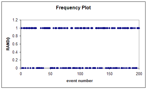
As an example of this, let us consider a coin toss. Now a days we can easily produce a simulation of an ideal coin toss experiment on a a computer using simple spreadsheet programs. (Remember computer simulations from the last topic, Measurement? Well, here we will create our own simulation!) Below is a frequency plot that I generated using Excel spreadsheet. In one column I entered the "event" numbers; starting with 1 and up to 200, so that each of these events represents one coin toss. Then in the next column I entered the function: =ROUND( RAND(), 0). This generates a random number between 0 and 1 that is rounded to zero decimal place, i.e. the outcome is either a 0 or a 1. The plot shows these values for the 200 events:

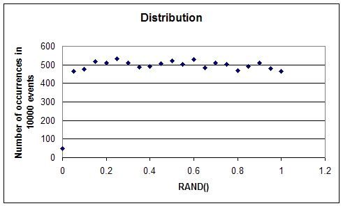
Now, if we count how many of these events produce a 1 and how many produce a 0, we find that in fact for the above graph 96 events are 1s and 104 events are 0s. That is to say, almost half as many events are 1s (say heads) and almost half as many are 0s (tails). The scheme that Excel uses to generate these numbers is called a pseudo random number generator. This is because it really uses an algorithm to create these numbers; so this process is deterministic in nature and exactly repeatable. But, evidently, one can prove mathematically that the sequence of numbers generated this way is fairly random. What do we mean by this?  It makes little sense to speak of distribution of a sequence of zeros and ones. That is just the number of zeros and number of ones in the sequence. But if we were to generate a sequence of numbers between 0 and 1, say within two decimals, then we could examine to see how the bins (0-0.01, 0.01-0.02,0.02-0.03,...,0.99-1.00) get occupied; i.e. how many of these random numbers occur with values in a given bin. The plot of the number of occurrences for each bin versus the bin values is then the distribution graph of this sequence of random numbers. If this graph is flat, the distribution is said to be a uniform distribution. In a uniform distribution all bins get filled equally.

Above graph shows the number of occurrences of random numbers generated by Excel's built in function, RAND(), counted over 20 bins from 0 to 1 : 0.0-0.05,0.05-0.1,...,0.95-1.0. (For this I used ROUND(RAND(),2) to generate 10,000 numbers from 0 to 1, each with two decimals. Then I used the FREQUENCY function of Excel to generate the number of occurrences. If you try this, be a bit patient. The calculation could take a minute or so.) It is clear from the above graph that in spite of the slight variations, the distribution function is flat.

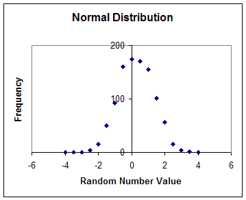
Random numbers need not to have a flat distribution function. In fact, it turns out that most random events in nature don't. The most common distribution function is called the normal distribution. The functional form of this distribution is Gaussian, or otherwise known as the Bell Curve. Why this is so, no one seems to know for sure; it appears to be a law of nature.

The above graph shows distribution of a sequence of1,000 random numbers that were generated using Excel. Here the numbers range in value from -4 to +4. I generated these using the Tools menu and then chose random number generator. But this time the sequence of random numbers don't have values that occur uniformly over its range. Instead, most of these random numbers have a value near the center of the range (zero). The further we move from this "most likely" value, the fewer these random numbers get. It appears, in fact, that none of the 1,000 random numbers have a value of either -4 or +4.

In the option that I used to generate these "Normally distributed" random numbers I could have specified how sharp I wanted the random numbers distribution to be. When I choose the distribution to be sharper, then most of the numbers in the sequence would have a value near the mean (here, zero). The measure of sharpness of the Gaussian distribution is signified by one of its parameters. This parameter is called: "standard deviation" and is a measure of the width of the distribution graph.

The analytical expression for the Gaussian function, f(x), is:

In this expression A is the maximum value of the function and is known as the amplitude, μ is the value at the mean (above example had this value to be zero), and σ is the standard deviation.

Notice that in our graph of our 1,000 random numbers very few have a value larger than 2. This means that the likelihood that any of these numbers chosen by random would have a value of 2 is small. If the values of our measurement were to show a random variation that followed a Gaussian distribution, then we see that the value of the standard deviation signifies two rather important feature of our experiment. First, the smaller the standard deviation, the most reliable is our result. Second, that the likelihood of a new trial to end up yielding a result different by more than one standard deviation from the mean will be very little. So, we can use the value of the standard deviation as a measure of the uncertainty of our results, i.e.

x_result = μ ± σ

Propagation of Errors

How do scientists and science practitioners estimate the uncertainty in the result of their experiment? Even though there is no one exact answer to this question, most procedures use the general guidelines developed by mathematical statistics (specifically probability distributions) to come up with a final answer. For a complete description of uncertainty estimation see the Uncertainty of Measurement pages of the National Institute of Standards and Technology (NIST).

In order for us to get a feeling for this, let us try a simple exercise. Let us imagine that we want to determine the value of the surface area of the desk that we are using. For this determination we need to measure the width and the length of our desk, say with a meter stick that is 1.00 m long and is calibrated in mm increments. The following (made up) table could be a reasonable table of data for such a measurement:

Notice that in the above table W and L represent the width and the length, respectively. While δW and δL are the absolute value of the difference between each measurement and the average value of the 10 trials for the width and the length measurements, respectively; i.e. the average deviation values. Strictly speaking, instead of the average deviation we should use the standard deviation as the measure of our uncertainty for either of these two directly measured quantities. After all, if we are assuming that our measurements of the widths and the lengths are "random", then we should expect that their frequencies follow a Normal distribution, for which the standard deviation is the agreed upon measure of its sharpness. But for the sake of simplicity of calculation, the average deviation is not an unreasonable substitute. In either case, the important question that we have not yet faced is how do we calculate the area of the table and how do we determine the uncertainty in its value?

One answer to this question could be that we should calculate the value of the area for each trial, and then use the average of these along with its value of average (or standard) deviation for our final result. The major shortcomings of this simple method is that, at the end, we would not know how the uncertainties of our separate measurements have affected the final uncertainty in our value of the area. This, in fact, is a serious deficiency, because it would not allow us to improve on our future measurements. It is hard to see this point in the context of the above oversimplified example, but for most experiments in which several different variables (say length, mass, temperature, etc.) are measured it is very important to know the sensitivity of final result on each of these variables. It is with this knowledge that we could improve on future measurements.

It takes a good deal of mathematical analysis, in the field of Statistics, to come up with a way of estimating the error in the final (calculated) result (here the area) using the uncertainties in the directly measured variables (here W and L). But fortunately for us most of the labor has already been done by others. (Again, see the section on error estimation at NIST's web site for a simple, but very useful example). What remains for us to do is to understand how these "formulae" have been arrived at. In particular, we need to know what are the assumptions that are used in these derivations.

Below is a quotation from the above referred to site published by NIST:

"Meaning of uncertainty If the probability distribution characterized by the measurement result y and its combined standard uncertainty u_c(y) is approximately normal (Gaussian), and u_c(y) is a reliable estimate of the standard deviation of y, then the interval y ­ u_c(y) to y + u_c(y) is expected to encompass approximately 68 % of the distribution of values that could reasonably be attributed to the value of the quantity Y of which y is an estimate. This implies that it is believed with an approximate level of confidence of 68 % that Y is greater than or equal to y ­ u_c(y), and is less than or equal to y + u_c(y), which is commonly written as Y = y ± u_c(y)."

Notice that the primary assumption is that the variable of measurement is Normally distributed. If that is the case, then it appears that by specifying the value of its uncertainty we are, in effect, stating that within certain limit of confidence (68%) the new (identical) measurements will produce the results that fall within the range of our estimated uncertainty. Of course, even though our 68% limit is fixed, we could, in principle, come up with an improved measurement that produces a smaller uncertainty. The smaller the uncertainty, then, the most likely that our average value is "the true" value; albeit our confidence level is fixed at 68%.

The next question we need to answer is how small could we make the error? Could we reduce the experimental error to zero? We will examine this question in the next section: Heisenberg's  Uncertainty Principle.