Heisenberg Uncertainty Principle

Fourier Transform

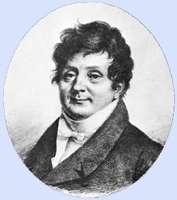
Baron Jean Batiste Joseph Fourier

What is even more fascinating is that it is possible to play the same game for continuous functions! That is, there are basis functions that span the whole of the function space. One of these basis sets, it turns out, is the (infinite) set of trigonometric functions of varying frequencies; the so called Fourier sine and cosine series, after the famous French mathematician Baron Jean Batiste Joseph Fourier.

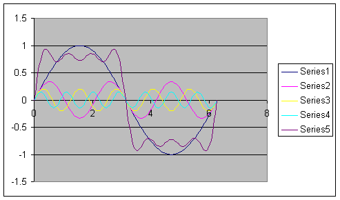
As an illustration of this mathematical representation, below is an Excel generated graph that shows five separate functions. The first four (series 1 through 4) are just sine functions whose frequency increases as their amplitude decreases. The last function, depicted as series 5, is just the sum of these sine functions. Notice that this sum is almost like a square-wave of the same frequency as the one shown in series 1. In fact, you can show that if you keep adding more and more of these sine functions (there is a specific formula that they must follow) the sum gets to be a better and better square wave. The expression, in fact, is:

f(ωt) = sin(ωt) + sin(3ωt)/3 + sin(5ωt)/5 + sin(7ωt)/7 + ...

This will generate a square wave function, f, of frequency ω. The more terms you include, the less wiggles on the flat parts. In practice, you will find that after ten terms or so new changes (improvements) happen very slowly!

Another major mathematical scheme that is named after Fourier is the so called Fourier Transform. This is an operation that connects two separate worlds of functions: those that belong to the frequency world with those that belong to the space world! Any given function in the frequency world (a function of frequency) is connected with, or if you will transformed into, a specific function in the space world (i.e. a specific function of space). In a one-dimensional case, the space variable could be x and the frequency variable, say ω_x. Given a function of space, say f(x), this Fourier transform then will generate a new and unique function, g(ω) using it. So, we could either "talk about" f(x), or about its frequency representation, g(ω). For example, f(x) could represent the size of an obstacle that we place in front of the path of a ray of light.

One interesting example of Fourier Transform is that of a Gaussian function. It turns out that the Fourier Transform of a Gaussian function is also a Gaussian, of course in the sister domain. So, for example, when we send our laser light through a small pin hole, the intensity of the light varies as a Gaussian (two dimensional) as a function of space. Thus the light's intensity is greatest at the center of the light pattern and drops off as the exponential of the square of the "distance" away from the center. If we check the frequency dependence instead, we'll also find a Gaussian relation.

In optics, a simple lens can create a Fourier Transform. So, if we begin with an image which a Fourier Transform of a picture, say a dog's, this will look as intensity variations that do not appear to have any resemblance to a dog. But once we send the light through a lens, we could recreate the image of the dog! Such a two-dimensional Fourier Transform, is called a Hologram.

Aperture & Frequency

One of the most interesting examples in physics that follows the description of Fourier transform is the relationship between frequency (or, if you like, wavelength) and an aperture, i.e. a pinhole. Although Fourier originally applied his mathematical theory to the study of heat, it turns out that this mathematics is useful for all wave or wave-like phenomena.

In the study of Optics we have known, since the 1800s, that light is simply an electromagnetic wave. In the visible region the wavelength of light determines the quality that we perceive as its color. Red light has a longer wavelength than blue light, for example. Because the wavelength and frequency are directly related, then we could equally associate the color of light with its frequency. It turns out that the frequency representation of light (really any wave, according to Fourier's mathematics) is related to its spatial presentation. In particular, when we know the light's spatial function, then we also know its frequency function. More over, whatever we do that affects the light's spatial properties, it will also affect its frequency. This may not seem, at first, interesting but a little reflection will convince us that this connection is a bit odd! The oddness is because we can measure the light's spatial properties and, seemingly independently, its frequency properties.

For example, consider light that is send through a prism. Because different wavelengths bend at different angles once light passes from air-to-glass-to-air, the prism acts as an analyzer. As a result, if our light was originally made of say red and green colors, these colors separate once the light goes through the prism and we will see a red light and a green light. In a sense, then, our frequency determination (separating the red from the green) has affected the light in a spatial way - it has made the red go in a different path than the green.

Now, what happens if we affect the light spatially, and in a periodic way; say by chopping it? Well, this periodic spatial restriction in fact causes a change in the light's frequency function. In a way, the color of light changes! In another non-periodic spatial restriction, one in which we restrict the path of light say by forcing it to pass through a pinhole, the light's frequency variation spreads in space. If we then collect a small portion of this spread light, this narrower spread will have a "purer" frequency. We call this process "spatial filtering" because we can use it to filter the light's frequency via purely spatial considerations. Another example of this filtering is in the use of single mode optical fibers as frequency limiting devices. See the section on Sydney VisLab Web pages on Fourier Optics.

When we consider how light is created , as particles called photons, it is difficult to accept this inter-connect of space and frequency domains. Is it that the aperture absorbs one "color" photon and re-emits it in such a way to create the observed frequency spread? Equally disturbing is when we observe wave like behavior exhibited by other particles, such as electrons, protons, neutrons and the like. For a simulation of these, try the following applets created by Professor Zoltan's group. Notices that these simulations recreate what real experiments have shown us to be the case in the laboratory.

Try Applets on Single-Slit experiment on the Visual Quantum Mechanics and Double-slit by Kansas State Group.

Heisenberg Uncertainty Principle

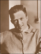Click on Heisenberg's AIP photo to visit The American Institute of Physics' History Center site.

Early in the development of quantum theory it was postulated that particles can be formulated as waves. This formulation was developed because in laboratory experiments it was discovered that particles such as electrons exhibited wave properties of diffraction and interference. In quantum theory the wave description is an abstract presentation, and not a direct quantification of a physical property. Because of this, the quantum waves are not themselves measurable. This is in contrast with the standard (classical) wave description of physical phenomena in which wave properties are measurable. For example, in a classical wave, say a sound wave, the amplitude of the wave is the measure of its loudness and its frequency is the measure of its pitch. Both of these properties can be measured in the laboratory in order to quantify the sound wave. In contrast, the wave associated with a quantum particle has no physical meaning by itself. But the knowledge of this purely theoretical function (the particle's wave function) is necessary for predicting values of the particle's measurable properties. So, to determine (predict) the particle's position or velocity, to name a few measurable quantities, we need to know its wave function.

Heisenberg's uncertainty principle is a direct consequence of this wave formulation and the fact that waves seem to connect separately measurable domains together! In its most commonly quoted form, Heisenberg's uncertainty principle connects the "position domain" with the "momentum domain". But there are other "sister" domains that are also interconnected; such as time and energy. In particular, Heisenberg's Uncertainty Principle states that the product of the uncertainty in one variable with the uncertainty in the other variable has a fixed lower limit. In terms of an equation, it states: (Δp)(Δq) cannot be smaller than h, where Δp is the uncertainty is the measurable p and Δq is the uncertainty in the measurable q, and h is some fixed (universal) constant (named after Planck; in SI system of units its value is 6.63x10-34). What does this mean?

In the earlier section discussing statistics we saw that when the influences of systematic errors (those connected with our method of measurement, including instrumentation) are minimized, there still remains a purely random error. This random error, as it turns out, always has a Normal (i.e. a Gaussian) distribution. The width of this distribution is our measure of the uncertainty in our measured result. Better methods and better instrumentations can lead to narrower and narrower widths of the error distribution graph and thus give us more accurate results. This, in fact, is the aim of many "precision" measurements. In the case of physical constant, for example, the National Institute of Standards and Technology (NIST) gives a yearly grant to investigators who can make a better measurement. Visit NIST's Precision Measurement Grant Information site and note that recently one of these grants was awarded to make an even better measurement of a familiar constant, the universal gravitation constant G.

So, when we say that the uncertainty in measurement of one variable (say position) is related to the uncertainty in the measurement of another variable (say momentum) we are really speaking about the widths of the error distributions of these two measurements. That is to say, this principle states that if we perform an experiment which manages to measure one of these variables with high degree of accuracy (i.e. very narrow width for its error distribution), then the error in the sister variable will be large (i.e. the width of its distribution gets larger).

Is this because our measurement of one variable, say the position x, causes a change in momentum px, i.e. the sister variable's value. The answer to this question is that this principle makes no statement of cause and effect! It just states that one cannot measure values for these sister variables with unlimited accuracies. Further more, these uncertainties are related as quoted in the above "equation". To state that x measurement causes or interferes with the momentum measurement is an inference beyond the statement of the Heisenberg Uncertainty Principle. It is, however, fair to ask why is there such a connection. Said differently, why is there the Heisenberg Uncertainty Principle? But we've already answered this question, albeit with a troubling outcome! It is a consequence of the wave description in quantum theory. Because all of our measurements to date agree with this description, we could then state that this uncertainty principle is simply the consequence of the way nature behaves. If we wish, then we could go a step further and infer that perhaps there is no independent (self existing) reality in the values of our interconnect measurables!

Is this just a conjecture (Natural Philosophy), or does it have any measurable consequences (Physics)?