The Plot Beam Tool
In general, before making measurements with an interferometer one should be familiar with the important characteristics of the individual antennas. One such characteristic about the VSRT interferometer which you will need to know for the subsequent labs is the width of the beam of each feed. The beam of the individual antennas that make up an interferometer is called the primary beam. Sources in the sky which are located away from the center of the primary beam can still be detected but the detected flux density will be decreased by a factor equal to the primary beam sensitivity at that position. When using an array of antennas to obtain an image of radio sources, the primary beam of the individual antennas essentially provides an upper limit to the field of view of the image, since radio emission coming from directions outside the primary beam will appear fainter, if detected at all.
What is "the Beam"?
Get Familiar with VSRTI Plotter
Lab Using the VSRT Interferometer
Analyze Data from VSRT Interferometer Beam-Pattern Lab
Examine Beam Pattern Without Data
Introduction: What is The Beam?
The beam is a radio astronomer's term to describe the angular area on the sky in which radiation will be detected by the radio telescope. The term derives from the fact that radio telescope
engineers design the telescopes as if they are transmitters.
The path of light can always be traced backward as well as forward and so modeling the radio telescope as a transmitter works, and is generally easier. Thinking of the telescope as
a radio transmitter, then, radio waves would be beamed outward through a finite angular area. Now, in terms of the telescope as a receiver of radiation, it will respond to the radiation coming in along that same beam. So, "the beam" of a telescope is a measure of how large an angular area the telescope is sensitive to. In general, a smaller telescope has a wider beam.
Now, the sensitivity of a telescope is not uniform across the beam. In most cases, the telescope
is most sensitive to radiation entering the telescope straight-on, and the sensitivity fades off
towards larger angles. So, radiation that enters in the beam but off-center might produce
a response in the receiver 80% of that when it enters in the very center.
The "width" of the beam is generally considered to be the angle between the half-maximum points
(or Full-Width-at-Half-Maximum, a.k.a. FWHM).
The width of the beam is also a measure of the
resolution of the telescope; if an individual telescope is used to map a source -- by charting the amount of radiation detected when the telescope is pointed in various directions -- then the inferred map cannot show details smaller than the beam size.
Obtaining the Data with the VSRT Interferometer:
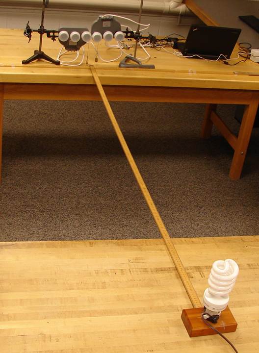
1. Place the feeds as close to each other as possible and place
a single helical CFL, standing on its end, at a distance of about 2 meters and in line with the midpoint between the feeds, as shown in the figure. To prevent reflections, place the feeds and CFL on the edges of different tables and make sure that there is no wall close behind the CFL. Turn off the room lights.
2. Check the ōpointingö of each feed by altering its pointing
direction while watching the signal in the single scan spectrum.
Adjust the pointing direction of the feeds one at a time to ensure that you get the maximum signal when the CFL is at the 0o position.
3. Press the ōrecordö button, and give the file a name that contains a pair of single quotes with the number æ0Æ inside the quotes. For example, the file name can be: PlotBeam`0'_15Sep. For this file, the æ0Æ means that these measurements correspond to an angle of 0o. (Note: It is very important that the file name contain the single quotes with a number inside. The VSRTI_Plotter program will look for the single quotes as its way of reading in the value of θ.)
4. While the data is recording, watch the screen and stop the
recording after about 50 scans by clicking "record." (Don't be concerned that the average spectrum window continues to integrate -- this window is separate from the recording of data into a file.) Take note of the antenna temperature and rms.
5. Keeping the distance of the CFL from the mid-point of the feeds roughly constant, move the CFL along an arc to a different position. Do not turn the feeds to keep them facing the CFL. Measure and record the angular position of the CFL relative to the midplane of the baseline. This is most easily accomplished using a little trigonometry, i.e. by measuring the perpendicular distance of the CFL from the mid-plane line, dividing by the distance of the CFL from the feeds and finding the inverse sine. See figure.

6. Click on record and give the same file name as before but with the new value of the angular position of the CFL in degrees between the single quotes. Record for about 50 scans.
7. Repeat steps 5 and 6 for all angles from -45o to +45o in steps of 5o. Increase the integration times as you get to larger angles - use about 60 scans for angles above 12o and about 100 scans for angles above 20o . At the larger angles, the signal will get weaker and so you'll want a smaller uncertainty to increase the signal to noise.
8. Put all your data files into a single folder.
Analysis of Data:
1. Open VSRTI_Plotter and select "Plot Beam."
2. Open the folder containing your data files, select all the data files, and drag-and-drop the whole set into the "data files" box on the right of the VSRTI_Plotter window. A plot of your data should appear instantly on the left.
2. Select ōShow Beam Patternö. YouÆll instantly see a curve representing the theoretical beam pattern for an antenna with the specifications set in the boxes to the lower right.
3. Try different values for "D," click "Update," and note how the model curve's width changes.
4. Note that the bottom of the curves donÆt match up. This is because of noise in the system...youÆll never get a zero signal, even when there is no source to detect. So, adjust the ōnoiseö level until the theoretical and observed curves match at the bottom. You can then adjust ōDö some more until the model curve matches the data.
5. When the curves match as best that you can make them, note the value of ōD.ö This is your measured value of the effective diameter of the feeds. For comparison, use a ruler to measure the physical diameter of each feed. How does this compare with your inferred effective D?
6. Save the plot as a JPEG file by moving the mouse cursor to the plot screen and right click.
7. Note the full-width-at-half-maximum (FWHM) of the beam pattern. This is the primary beam width of the VSRT feeds.
8. Convert your primary beam width to radians and compare with that given by
Beam(FWHM) = 1.22 λ/D,
where D is the diameter of the antenna and λ is the wavelength (2.5 cm) of the radiation.
9. Play with the value of ōDö and note how it changes your beam pattern. Now adjust λ and note how the beam pattern changes. Note, in particular, how the width of the beam depends on λ and D.
Examination of Beam Pattern Without Data:
If you don't have a VSRT Interferometer or any data, you can still use this tool to explore how an antenna's beam depends on the parameters. Click on "Show Beam Pattern", and adjust the values of "D" (the diameter of the antenna) and λ
(the wavelength of the radiation), click "Update" after each change, and see how the beam pattern changes. Measure the FWHM of the beam pattern and compare to that given by
Beam(FWHM) = 1.22 λ/D.
To save the plot as a JPEG file, move the mouse to the plot screen and right click.