The VSRTI_Plotter Tool
VSRTI_Plotter is designed as a tool for facilitating the analysis of data using the VSRT ("Very Small Radio Telescope") Interferometer for labs introducing the basics of aperture synthesis. This tool is also useful for simulating these experiments for users without the equipment. If not yet familiar with the controls in this tool, read the "Controls and Buttons for the VSRTI Plotter Programs" first.
Instructions for the labs are
linked below.
Controls and Buttons for VSRTI_Plotter Programs
1. After clicking on the "VSRTI_Plotter.jar" shortcut, you'll see a small pop-up window appear like that shown in Figure 1 below.
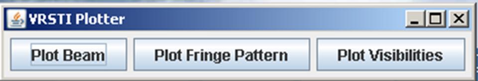
Figure 1: The first window to appear in the VSRTI Plotter package.
The window contains three options "Plot Beam," "Plot Fringe Pattern," and "Plot Visibilities." (Do not do the "Plot Fringe Pattern" lab.) For now click on "Plot Beam," which will open a new display like that in Figure 2. This new window contains a graph on the left and on the right you'll see a box for "Data files" above a number of input boxes and control buttons.
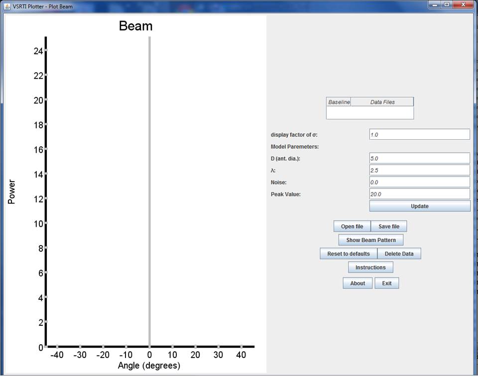
Figure 2: The display when running Plot Beam in the VSRTI_Plotter package.
2. As you move your mouse over the input boxes you should see ōtool tipsö appear. These tips give brief statements about
each control.
3. To read-in VSRT Interferometer data files, simply highlight and select all the relevant data files and drag-and-drop them into the empty "Data files" box. You can add and delete data files at any time. NOTE: All the data file names must
contain a pair of single quotes with the value of the indendepent variable for that lab
(θ for Plot Beam, for example) between the quotes.
DO NOT use the ōOpen fileö button to read in raw data. This button is used to read in
files saved with "Save File", as explained below.
4. The boxes immediately below the data-files box are the input parameters, which you can adjust. After changing an input parameter, click on "Update."
5. The size of the displayed error bars is equal to the uncertainty in the data multiplied by the ōdisplay factor of σö. (The uncertainty is calculated as
√ rms/N
, where rms is the measured root-mean-square of the deviations
in the data file and N is the number of values in the average). The rms values
tend to be small with the VSRT interferometer and so the errors bars will generally be too small for the
display without the display factor. If you have large error bars, you can change the display factor of
σ using the input box.
6. The ōShow ... ō button displays a theoretical curve for that lab. The curve depends
on some of the input parameters and so will change when you adjust these parameters (and click "Update"). This curve can be used both to fit your data by eye, leading to conclusions
regarding the values of the input parameters, and to demonstrate the concepts of the lab without data.
7. The "Reset to Defaults" button returns all input parameters to the default settings.
8. You can read the x,y values of a data point in the graph by moving the mouse cursor onto the data point and waiting a moment for the values to appear.
9. When you get a plot that youÆd like to save, you can right-click on the graph and save the image as a JPEG or eps file.
10. At any point, you can click ōSave Fileö, which will save the data into a three column ascii file. This file will have a different format from the .rad file written by the VSRT Interferometer software. Files ōsavedö by VSRTI_Plotter can be read back in using the ōOpen Fileö button. DO NOT drag and drop VSRTI_Plotter saved files into the data files box...that box is strictly for data files written by the VSRT Interferometer software.
11. To delete a data point, click on the appropriate data file in the "data files" box and hit the "delete" key.
12. Comments about units: The equations used for the models in "Plot Beam" assume the user has calculated the position angles of the CFL in units of degrees. However, in "Plot Visibilities," the angle input parameters (angular sizes of sources and angular position of second source) are in units of radians. (The expectation is that students would more naturally measure angles in degrees in the first two labs, while in the Visibilities lab inferring the angles in radians is more meaningful in terms of understanding the relation between the Visibility function and the intensity distribution of the light source.)
Also, the default setting for the wavelength of the detected radiation is in cm, and so all other distance values (such as the diameter of the feed, or the distance between feeds) is in cm. If one wishes to measure these distances in another unit, then the setting for the λ input box should be changed accordingly.
Links to Labs
Plot Beam
A lab demonstrating the resolution of a radio telescope, and the "primary beam" of an intereferometer antenna.
Plot Visibilities Labs
Used for three labs which introduce the concept of "Visibilities" and demonstrate how the "shape" of the Visibility funcition relates to the structure of the source.
Exploration of Fourier Transforms Lab.
First, Go to http://minerva.union.edu/marrj/radioastro/labfiles.html, download TIFT.zip, and extract all the files. Go into the TIFT folder and make a shortcut of TIFT\_Chooser.jar on your desktop. Open TIFT\_Chooser.
Then follow the instructions at
this link