The Plot Visibilities Tool
Get Familiar with VSRTI Plotter
What are Visibilities?
Lab: Observations of A Single Resolve Source
Lab: Observations of A Pair of Sources
Lab: Observations of A Mystery Source
Additional Notes Regarding the VSRT Interferometer Lab
Introduction: The Visibility Function (a.k.a. "Visibilities")
When radio astronomers use an array of antennas to make an image of a radio source, each pair of antennas acts as an interferometer. And, the data used to make the images are the outputs from the interferometers as a function of the interferometer ``baseline'' -- a vector defined as the distance between the antennas and their relative orientation. The response of each interferometer also depends on the direction of the radio source in the sky and on the shape and size of the radio source. The dependence on the direction of the radio source is called the fringe function, and is a well known function. The dependence of the detected signal on the source structure, as a function of baseline divided by the wavelength, is the "visibility function," V(b/λ). Note that the independent variable is not simply baseline, but baseline divided by wavelength.
In professional radio astronomy interferometric observations, the fringe function is removed from the data leaving only the visibility function. In this lab, we place the source in line with the center of the baseline and keep the source at that position. The fringe function, then, does not come into play, and so the response of the interferometer is purely the visibility function. To obtain the visibility function, you will need to make measurements with a range of baselines.
Also, to keep the lab relatively simple and straight-forward, we
only measure the visibility function in one dimension. Our visibility function, therefore, is easily displayed in a simple graph, and is shown in the graph window at the left side of the VSRTI_Plotter window.
A. Observations of a Single Resolved Source
When observing a source with a large angular size, the radio waves enter the antennas over a range of direction angles, which causes a decrease in the combined signal from the two antennas.
This decrease is more pronounced for antennas that are further apart. As a result the total detected power on longer baselines for a large source will be less than that from a smaller source with the same total flux density. And, similarly, interferometers with longer baselines are more sensitive to the source's angular size. A shorter-baseline interferometer, therefore, will have less of a decrease in the detected power than will an interferometer with a longer baseline. This effect is commonly described by saying that the longer baselines "resolve out" some of the flux of the source. And, the longer the baseline, the more of the flux is resolved out.
By plotting the visibilities (from a source located at θ = 0) for a range of baseline distances one can, then, infer the angle over which the flux density of an extended source (i.e. not a point source) is distributed.
In this lab, you will obtain and plot the visibilities vs. baseline and discover the baseline-dependence of the detected power, revealing that the CFLs are not really point sources.
Procedure
1. Place a thinner CFL (e.g. a straight-tubed CFL), standing on end (to give it a regtangular profile), at the mid-plane position (θ = 0).
2. Place two metal sheets slightly in front of the CFL by about a few cm, but with a gap equal in width to the CFL (about 4.5 cm if using a straight-tubed CFL) for the radiation to pass through, as shown in the figure. The metal sheets should be tall enough to reach the top of the CFL; paper clipping two pieces of scrap aluminum to metal book ends works well. (The metal sheets are used to address the three-dimensionality of the CFLs.
notes at the end for more discussion.)
The gap between the edges of the metal sheets should be 2 meters from the feeds

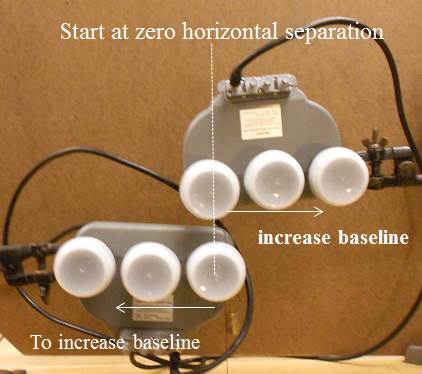
3. Start by placing the feeds one above the other (so that their horizontal distance is zero), as shown in the next figure. Make sure that they are exactly the same distance from the CFLs. To prevent reflections, place the feeds and CFLs on the edges of different tables and make sure that there is no wall close behind the CFL. Turn off the room lights.
4. Click �record�, and in the file name type �0� between the quotes, to represent a baseline distance of 0. Record for about 50 scans.
5. Move the feeds to a horizontal separation distance of 2 cm by moving each of them 1 cm in opposite directions. Click "Record," use the same file name but with '2' between the single quotes.
6. Increase the separation distance of the feeds by another 2 cm. Keep the distance of the feeds from the gap constant by moving them along an arc centered on the gap. Also, take care to ensure that the feeds are exactly the same distance from the CFL and turn the feeds slightly as you move them so that they are always aimed directly facing the gap. Click �Record,� and put the new value of the baseline distance in cm between the single quotes.
7. Repeat the last step, always increasing the separation distance of the feeds by 2 cm, up to a separation distance of 60 cm. (See
notes at end for a discussion of the maximum baseline you can use.) When the detected power gets below 15 K, increase the integration time to 100 scans.
8. Replace the narrow CFL with a wider CFL (such as the 55W helical CFL) and widen the gap to match the width of the new CFL (about 7.5 cm). Repeat the above experiment. Save the data into files with a different name (and/or store in a different folder).
Analysis of Data of a Single Resolved Source
1. Open VSRTI_Plotter, and click on "Plot Visibilities." Drag-and-drop the data files for the set-up with the narrower gap into the data files box. You should see a graph of detected power vs. (baseline distance divided by λ) that decreases with increasing distance.
2. Click on "Display Model Visibility", set T2 = 0, and for "shape1" select "rectangular." Adjust the values of T1 and Φ1 until the curve fits the data. (See
notes at end for a discussion of the model.) The value of Φ1 is the apparent angular size of the CFL in radians according to the data. This implies a linear size, l, of the CFL of
l = Φ d
where d is the distance of the CFL. (Recall that a body�s apparent angular size in radians is approximately equal to its linear size divided by its distance.) If you followed the instructions here your distance, d is equal to 2 meters. Compare your inferred value of l to the linear distance between the metal plates used for that data set. These values should agree, within experiemental error.
3. Right click on the plot window and save a jpeg file of the graph.
4. Click "Delete Data" and then drag-and-drop the files for the data with the wider gap. How does this change the plot on the left? Don't worry about the absolute value of the measured power between the two plots, since they involved different lamps. Focus, primarily, on the difference in the shape.
5. Find the best fit value of Φ1 and again calculate the inferred value of l and compare with the actual setting.
6. Note that in this experiment, the CFL never moved relative to the midpoint of the baseline. In this experiment, therefore, the change in the measured power is not due to the same concept demonstrated in the "Plot Beam" lab. In this lab, the source was stationary, but the feeds were moved to different baselines. You measured the interferometer response as a function of baseline distance. This is called the "Visibility function." Discuss the shape of the visibility function for an observation of a resolved source and how this shape changes as the size of source is decreased.
7. By extrapolation, try to infer what the shape of the visibility function is for a point source. Test your answer by viewing the model curve ("Display Model Visibilities" button) when the value of Φ1 is set to 0 (remember to click "Update"). When the visibility function is such a shape, then no angular size of the source can be inferred and so this indicates when the source is unresolved.
8. Discuss why real interferometric observations of radio sources involve more than one pair of antennas. Consider the fact that with three antennas, for example, there are three pairs of antennas, and each pair can involve a different baseline. How does observing with a large number of antennas, such as with the VLA, provide the information needed for radio astronomers to obtain images of resolved radio sources?
(Hint: consider the graph you created to reveal the visibility function and how quickly the data for this graph could be obtained if you had more than two feeds.)
9. Consider, and discuss, the resolution of an array of antennas as it relates to the linear size of the array. Is an array which includes large baselines more or less capable than a smaller array of inferring the structure of a compact source. For an array with a range of baselines, which baselines determine the resolution -� the longest or shortest? Write a mathematical relation to determine the resolution angle of an array of antennas.
10. Consider if you observed a large source with a large array which involved only very long baselines (such as with VLBI). Explain why this situation might result in a null detection. It is, therefore, not a good idea to observe a radio source with an array with too good resolution. When planning an observation of a known source, you should pick the instrument whose resolution best matches your source.
B. Observations of a Pair of Sources
Observing a pair of sources that are separated by a large angle, relative to the resolution of the interferometer, is, essentially, combining the interferometer responses to sources at two different positions. As mentioned in the previous lab the interferometer response has a dependence on source position. In the same way that light passing through two slits produces a striped pattern with the distance between the stripes depending inversely on the distance between the slits, the visibility function of a pair of sources has a sinusoidal dependence on b/λ with a wavelength (or "spatial period") that is inversely proportional to the angular separation of the sources. By plotting the visibilities for a range of baseline distances one can, then, identify a binary source and determine the separation angle of the sources.
In this lab, you will use two CFLs to reveal the sinusoidal shape of the visibility function for two sources and show the relation between the angular separation of the CFLs and periodicity in the visibility function.
Procedure
1. Start with the feeds one above the other so that their horizontal separation distance is zero.
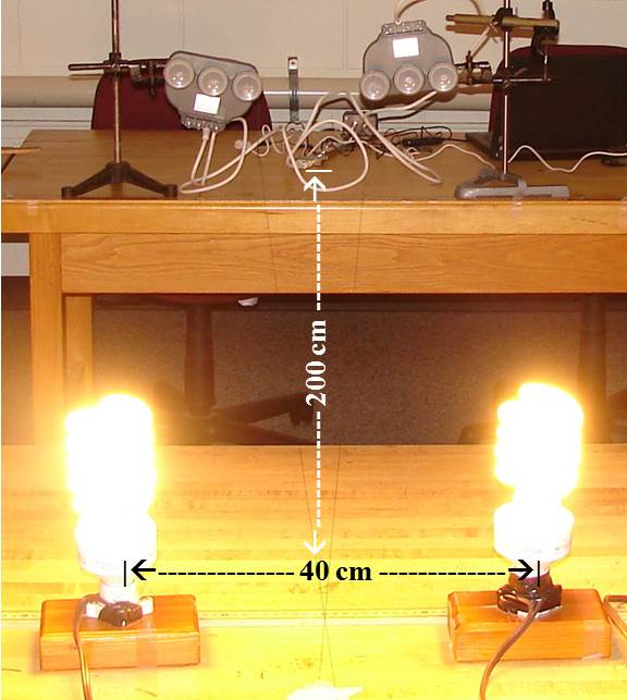
2. Place a pair of helical CFLs, standing on end, at a distance of 2 meters from the feeds, and separated by 40 cm in the perpendicular direction. Aim the feeds at the midpoint between the CFLs. A picture of the set-up is shown in the figure.
3. Click on �Record� and put a �0� between the single quotes in the file name. Record until n ~ 50.
4. Move the feeds to a horizontal separation distance of 2 cm by moving each of them 1 cm in opposite directions. Click "Record" and use the same file name with the '2' between the single quotes.
5. Repeat step 4, always increasing the separation distance by 2 cm, up to a final distance of 60 cm. (See
notes for a discussion of the maximum baseline you can use.)
Turn the feeds as you move them so that they are always facing the midpoint between the two CFLs and make sure that they stay the same distance from the CFLs. Click �record� and put the value of the baseline distance (in cm) between the quotes. When the antenna temperature gets below 30 K integrate for 60 scans and when it is below 15 K integrate for 100 scans.
6. Rearrange the CFLs so that they are separated by 30 cm and repeat the above procedure but make sure that the file names are different, and/or place them into a different folder. Obtain a third data set for CFLs separated by 20 cm.
Analysis of Data of a Pair of Sources
1. Open VSRTI_Plotter and select "Plot Visibilities." Drag and drop the data files for CFLs separated by 40 cm. You should see a quasi-sinusoidal function appear, whose amplitude decreases with baseline distance. The decreasing amplitude is due to the resolving of the individual CFLs, as you demonstrated in the observations of a single source. The oscillations, though, indicate that there is a second source, away from the θ = 0 position.
2. Measure the distance between peaks, in terms of b/&lamda;, in the sinusoidal function. Call this Θ. Calculate the angular separation of the CFLs from
θ(radians) = x/d, where x is the linear separation distance between CFLs.
3. Click �delete data� and then drag-and-drop the data set for CFLs separated by 30 cm, and measure the distance between peaks and calculate θ from x/d. Do the same with the data set for CFLs separated by 20 cm.
4. In a separate plotting program (such as Excel), plot Θ vs. θ. What is the relation between these two parameters? Do your data fit the relation
Θ = 1 / θ (radians)?
5. Drag-and-drop each data set into the data files box again. This time click on "Display Model Visibility" and set "shape1" and "shape2" to "rectangular." (Note: if you placed the CFLs on their sides, with the ends aimed at the feeds, then you should select "uniform disk" for the shapes.) Adjust the five input parameters (Φ1 and Φ2 are the angular sizes of each source, in radians, T1 and T2 are the radiation powers, in Kelvin, from each lamp, and θ is the angular position of the second lamp relative to the first, as seen from the center of the feeds baseline). See
notes at end for a discussion of the model.)
For your best fit models, write the values of θ, calculate the inferred linear separation distances of the CFLs using
x = θ d
and compare to the actual values you used in the set-ups.
6. As with the "Single Resolved Source" lab, the CFLs did not move relative to the midpoint of the baseline and so your
plot shows the visibility function. Discuss the shape of the visibility function for an observation of a double source and how this shape changes when the angular separation between the two pieces change.
7. Imagine planning an observation at a wavelength of 6 cm of a double radio source in which the sources are separated by 30 arcseconds. If planning an observation of this source, what ranges of baselines would be needed to map this double source?
C. Observations of a Mystery Source
[Note to instructors: If you wish to assign this lab and would like advice about how to set up a mystery source that is solvable, feel free to e-mail me (marrj@union.edu).]
Your instructor will have some number of CFLs inside a cardboard box. Your goal, now, is to use the feeds, at a range of baselines, repeating the procedure of the previous lab but with the CFLs hidden in the box, obtain a visibility function, analyze it, and make a model of what you think the "structure" of the mystery source is (how many CFL's and in what positions?).
Remember to keep in mind the main principles that were demonstrated in the previous two labs. How does the visibility function appear with a resolve source? How does the visibility function appear for a single pair of sources separated by a given angular distance? Extrapolation of these principles should help you to, now, infer a slightly more complex stucture. You cannot use the "Show Visibilities" button to help you in this lab, since the model to match the mystery source has not been put in.
Here are some principles from the previous two labs which you can use as hints for this lab:
1. As demonstrated in the single-resolved-source lab, the longer baselines resolve out more of the structure of an extended source. This means that the zero-baseline visibility should contain the flux from the entire source.
2. Each pair of sources produces a periodic visibility function with period given by Θ = 1/θ. Considering the principle stated in no. 1, each periodicity must have a maximum at the zero baseline...so to identify periodicities, start at b/λ=0 and look for the next peak after that.
Additional Notes
1. Model Equation
The model used in Plot Visibilities is given by
T = {TA2 + TB2 + 2TATBcos(2πbsin(θ)/λ))}1/2,
where the detected power of each individual CFL, as a function of baseline, b, if rectangular in shape, is
TA=T1(λ/(2πΦ1))√ 2 (1-cos(2πbΦ1/λ))
and
TB=T2(λ/(2πΦ2))√ 2 (1-cos(2πbΦ2/λ)).
If the source is a uniform disk, the detected power is given by
TA=T1[J1(πΦAb/λ) / (πθAb/λ)],
where J1 is the first order Bessel function of the first kind.
2. Maximum Baselines
The interferometric equations for the amplitude of the Visibility assume that the rays approach the feeds in parallel rays, which is clearly true for a source that is infinitely far away. For these labs, however, the CFLs are only about 2 meters away while the feeds get up to 10's of centimeters apart. The assumption of parallel rays, therefore, can break down if the feeds are put too far apart. The assumption of parallel rays is used in the derivation of the equation to assign the path-length difference, which causes the phase difference in the two feeds. For results of these labs to not be significantly altered by an error in the assumed phase difference, the difference between the model and true path length difference needs to be within 1/8th of λ, so that the model and true phase differences stay within π/4. This constraint is satisfied if
(bx/d){1-[1+(b/2d)2]-1/2} < 0.003
where b is the baseline distance, x is the largest linear distance between points of radio emission (i.e. the diameter of the CFL for the Single-Resolved Source lab, and the distance between CFLs in the Double-Source lab), and d is the distance along the mid-plane from the CFL plane to the feeds plane (d = 200 cm if following the instructions above).
For the Single-Resolved Source lab (in which x = 5 cm), one should keep the baseline shorter than 160 cm.
For the Double-Source lab, where the largest x is 40 cm, the baselines should be kept under 80 cm.
3. Apparent Angular Size of CFL's
When conducting the "Single Resolved Source" lab, if the metal screens are not used to set the width, the apparent size of the CFL will be larger than the CFL itself. This occurs because of the 3-dimensionality of the situation. The feeds detect radio emission from the back of the CFL as well as the front. As the feeds are moved to larger baselines, their view of the CFLs include the sides of the CFL. The effect is that the CFLs act like a larger source. For this reason, we recommend that the single resolved source lab be conducted with a pair of metal shields in front of the CFL to, effectively, make a slit with adjustable width. The shields block the radiation from the sides when the feeds move to larger baselines.